一、实验目的
1. 熟悉数据标注的流程,熟悉相关的函数;
2. 学习运用Python对手写数字图片进行数据标注,实现数据预处理;
3. 学习KNN,SVN,CNN三种网络模型分别对MNIST手写数据集以及手写数字图片数据集进行识别并计算预测准确率。
二、使用仪器、材料
环境:Python 3.12.4 (Anaconda3)

开发工具:Visual Studio Code
三、实验过程原始记录及实验结果分析
3.1处理MNIST手写数据集
3.1.1 KNN(K-近邻算法)
~~~
python代码:
import struct
import numpy as np
import matplotlib.pyplot as plt
import matplotlib
from sklearn.neighbors import KNeighborsClassifier
from sklearn.metrics import accuracy_score, confusion_matrix, classification_report
import os
import joblib # 用于保存和加载模型
# 设置中文字体以支持中文标签
# 请确保系统中安装了相应的中文字体,例如SimHei或SimSun
matplotlib.rcParams['font.sans-serif'] = ['SimHei'] # 设置中文字体为黑体
matplotlib.rcParams['axes.unicode_minus'] = False # 解决负号显示为方块的问题
# 定义读取IDX文件的函数
def read_idx_images(filename):
with open(filename, 'rb') as f:
magic, num, rows, cols = struct.unpack('>IIII', f.read(16))
if magic != 2051:
raise ValueError(f'无效的魔数 {magic} 在图像文件: {filename}')
images = np.frombuffer(f.read(), dtype=np.uint8).reshape(num, rows, cols)
return images
def read_idx_labels(filename):
with open(filename, 'rb') as f:
magic, num = struct.unpack('>II', f.read(8))
if magic != 2049:
raise ValueError(f'无效的魔数 {magic} 在标签文件: {filename}')
labels = np.frombuffer(f.read(), dtype=np.uint8)
return labels
# 配置文件路径
train_images_path = r'E:\CODE\DataMining\teamWork\dataset\mnist\train-images.idx3-ubyte'
train_labels_path = r'E:\CODE\DataMining\teamWork\dataset\mnist\train-labels.idx1-ubyte'
test_images_path = r'E:\CODE\DataMining\teamWork\dataset\mnist\t10k-images.idx3-ubyte'
test_labels_path = r'E:\CODE\DataMining\teamWork\dataset\mnist\t10k-labels.idx1-ubyte'
# 检查文件是否存在
for path in [train_images_path, train_labels_path, test_images_path, test_labels_path]:
if not os.path.exists(path):
raise FileNotFoundError(f'文件未找到: {path}')
# 读取数据
print("正在读取训练图像...")
train_images = read_idx_images(train_images_path)
print("正在读取训练标签...")
train_labels = read_idx_labels(train_labels_path)
print("正在读取测试图像...")
test_images = read_idx_images(test_images_path)
print("正在读取测试标签...")
test_labels = read_idx_labels(test_labels_path)
print(f"训练图像数量: {train_images.shape[0]}")
print(f"测试图像数量: {test_images.shape[0]}")
# 数据预处理
# 归一化图像数据到 [0, 1]
train_images = train_images.astype('float32') / 255.0
test_images = test_images.astype('float32') / 255.0
# KNN需要二维的输入,因此将28x28的图像展平为784维的向量
train_images_flat = train_images.reshape(train_images.shape[0], -1) # 形状: (60000, 784)
test_images_flat = test_images.reshape(test_images.shape[0], -1) # 形状: (10000, 784)
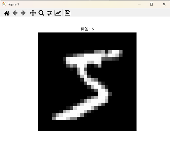
# 查看一张图像
plt.imshow(train_images[0], cmap='gray')
plt.title(f"标签: {train_labels[0]}", fontproperties='SimHei')
plt.axis('off')
plt.show()
# 构建KNN模型
knn = KNeighborsClassifier(n_neighbors=3, n_jobs=-1) # 使用3个邻居,n_jobs=-1使用所有CPU核心
# 训练模型
print("正在训练KNN模型...")
knn.fit(train_images_flat, train_labels)
print("KNN模型训练完成。")
# 评估模型
print("正在评估KNN模型...")
test_predictions = knn.predict(test_images_flat)
test_accuracy = accuracy_score(test_labels, test_predictions)
print(f"\n测试准确率: {test_accuracy}")
# 打印分类报告
print("\n分类报告:")
print(classification_report(test_labels, test_predictions, target_names=[str(i) for i in range(10)]))
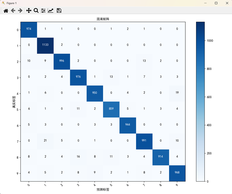
# 混淆矩阵
cm = confusion_matrix(test_labels, test_predictions)
plt.figure(figsize=(10, 8))
plt.imshow(cm, interpolation='nearest', cmap=plt.cm.Blues)
plt.title('混淆矩阵', fontproperties='SimHei')
plt.colorbar()
tick_marks = np.arange(10)
plt.xticks(tick_marks, [str(i) for i in range(10)], rotation=45, fontproperties='SimHei')
plt.yticks(tick_marks, [str(i) for i in range(10)], fontproperties='SimHei')
# 在每个单元格上显示数字
thresh = cm.max() / 2.
for i in range(cm.shape[0]):
for j in range(cm.shape[1]):
plt.text(j, i, format(cm[i, j], 'd'),
horizontalalignment="center",
color="white" if cm[i, j] > thresh else "black",
fontproperties='SimHei')
plt.ylabel('真实标签', fontproperties='SimHei')
plt.xlabel('预测标签', fontproperties='SimHei')
plt.tight_layout()
plt.show()
# 保存KNN模型
model_save_path = 'mnist_knn_model.joblib'
joblib.dump(knn, model_save_path)
print(f"模型已保存为 {model_save_path}")
# 加载并使用保存的KNN模型(示例)
# loaded_knn = joblib.load(model_save_path)
# example_image = test_images_flat[0].reshape(1, -1)
# example_prediction = loaded_knn.predict(example_image)
# print(f"加载的模型预测结果: {example_prediction[0]}, 真实标签: {test_labels[0]}")
~~~
运行结果:
终端输出:
PS E:\CODE\DataMining\teamWork\model> & E:/software/Anaconda3/python.exe e:/CODE/DataMining/teamWork/model/mnistKNN.py
正在读取训练图像…
正在读取训练标签…
正在读取测试图像…
正在读取测试标签…
训练图像数量: 60000
测试图像数量: 10000
正在训练KNN模型…
KNN模型训练完成。
正在评估KNN模型…
测试准确率: 0.9705
分类报告:
precision recall f1-score support
0 0.97 0.99 0.98 980
1 0.96 1.00 0.98 1135
2 0.98 0.97 0.97 1032
3 0.96 0.97 0.96 1010
4 0.98 0.97 0.97 982
5 0.97 0.96 0.96 892
6 0.98 0.99 0.98 958
7 0.96 0.96 0.96 1028
8 0.99 0.94 0.96 974
9 0.96 0.96 0.96 1009
accuracy 0.97 10000
macro avg 0.97 0.97 0.97 10000
weighted avg 0.97 0.97 0.97 10000
3.1.2 CNN(卷积神经网络)
~~~
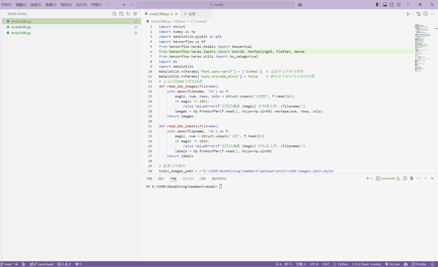
python代码:
import struct
import numpy as np
import matplotlib.pyplot as plt
import tensorflow as tf
from tensorflow.keras.models import Sequential
from tensorflow.keras.layers import Conv2D, MaxPooling2D, Flatten, Dense
from tensorflow.keras.utils import to_categorical
import os
import matplotlib
matplotlib.rcParams['font.sans-serif'] = ['SimHei'] # 设置中文字体为黑体
matplotlib.rcParams['axes.unicode_minus'] = False # 解决负号显示为方块的问题
# 定义读取IDX文件的函数
def read_idx_images(filename):
with open(filename, 'rb') as f:
magic, num, rows, cols = struct.unpack('>IIII', f.read(16))
if magic != 2051:
raise ValueError(f'无效的魔数 {magic} 在图像文件: {filename}')
images = np.frombuffer(f.read(), dtype=np.uint8).reshape(num, rows, cols)
return images
def read_idx_labels(filename):
with open(filename, 'rb') as f:
magic, num = struct.unpack('>II', f.read(8))
if magic != 2049:
raise ValueError(f'无效的魔数 {magic} 在标签文件: {filename}')
labels = np.frombuffer(f.read(), dtype=np.uint8)
return labels
# 配置文件路径
train_images_path = r'E:\CODE\DataMining\teamWork\dataset\mnist\t10k-images.idx3-ubyte'
train_labels_path = r'E:\CODE\DataMining\teamWork\dataset\mnist\t10k-labels.idx1-ubyte'
test_images_path = r'E:\CODE\DataMining\teamWork\dataset\mnist\t10k-images.idx3-ubyte'
test_labels_path = r'E:\CODE\DataMining\teamWork\dataset\mnist\t10k-labels.idx1-ubyte'
# 检查文件是否存在
for path in [train_images_path, train_labels_path, test_images_path, test_labels_path]:
if not os.path.exists(path):
raise FileNotFoundError(f'文件未找到: {path}')
# 读取数据
print("正在读取训练图像...")
train_images = read_idx_images(train_images_path)
print("正在读取训练标签...")
train_labels = read_idx_labels(train_labels_path)
print("正在读取测试图像...")
test_images = read_idx_images(test_images_path)
print("正在读取测试标签...")
test_labels = read_idx_labels(test_labels_path)
print(f"训练图像数量: {train_images.shape[0]}")
print(f"测试图像数量: {test_images.shape[0]}")
# 数据预处理
# 归一化图像数据到 [0, 1]
train_images = train_images.astype('float32') / 255.0
test_images = test_images.astype('float32') / 255.0
# 添加通道维度(因为CNN需要4D输入)
train_images = np.expand_dims(train_images, -1) # 形状: (60000, 28, 28, 1)
test_images = np.expand_dims(test_images, -1) # 形状: (10000, 28, 28, 1)
# 转换标签为独热编码
train_labels_categorical = to_categorical(train_labels, num_classes=10)
test_labels_categorical = to_categorical(test_labels, num_classes=10)
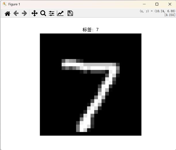
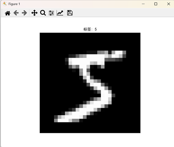
# 查看一张图像
plt.imshow(train_images[0].squeeze(), cmap='gray')
plt.title(f"标签: {train_labels[0]}")
plt.axis('off')
plt.show()
# 构建CNN模型
model = Sequential([
Conv2D(32, kernel_size=(3, 3), activation='relu', input_shape=(28, 28, 1)),
MaxPooling2D(pool_size=(2, 2)),
Conv2D(64, kernel_size=(3, 3), activation='relu'),
MaxPooling2D(pool_size=(2, 2)),
Flatten(),
Dense(128, activation='relu'),
Dense(10, activation='softmax') # 10个类别
])
# 编译模型
model.compile(optimizer='adam',
loss='categorical_crossentropy',
metrics=['accuracy'])
# 显示模型摘要
model.summary()
# 训练模型
history = model.fit(train_images, train_labels_categorical,
epochs=10,
batch_size=128,
validation_split=0.1)
# 评估模型
test_loss, test_acc = model.evaluate(test_images, test_labels_categorical, verbose=2)
print(f"\n测试准确率: {test_acc}")
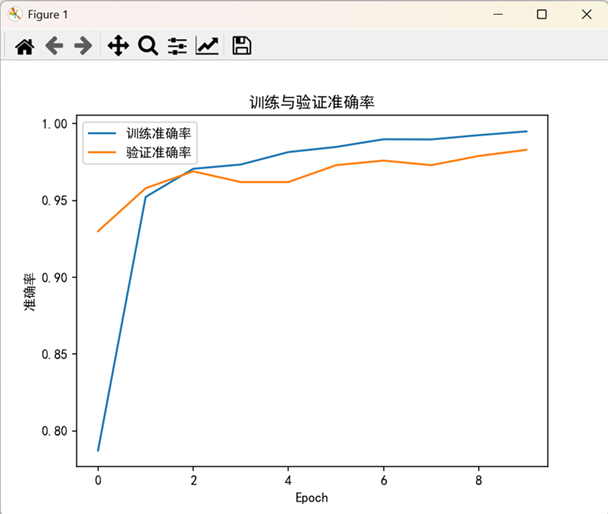
# 可视化训练过程
# 准确率曲线
plt.plot(history.history['accuracy'], label='训练准确率')
plt.plot(history.history['val_accuracy'], label='验证准确率')
plt.xlabel('Epoch')
plt.ylabel('准确率')
plt.legend()
plt.title('训练与验证准确率')
plt.show()
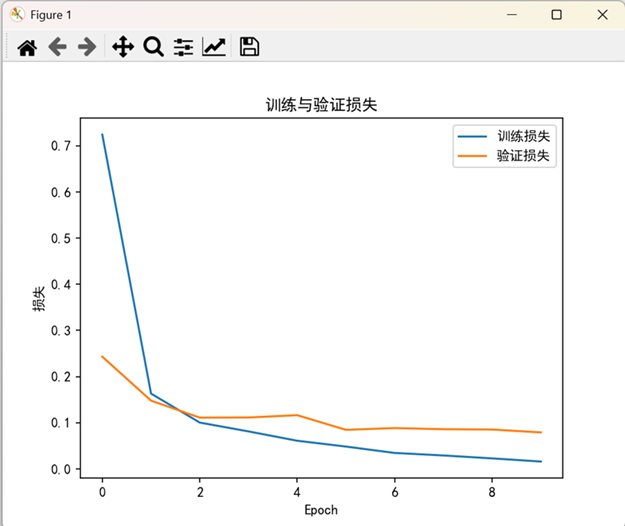
# 损失曲线
plt.plot(history.history['loss'], label='训练损失')
plt.plot(history.history['val_loss'], label='验证损失')
plt.xlabel('Epoch')
plt.ylabel('损失')
plt.legend()
plt.title('训练与验证损失')
plt.show()
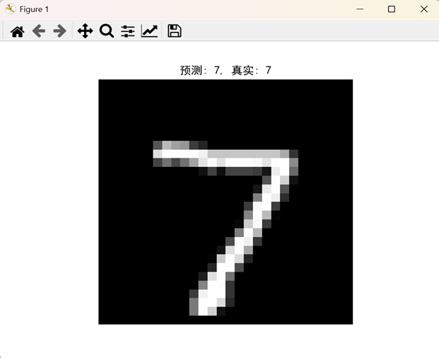
# 使用模型进行预测
predictions = model.predict(test_images)
# 显示测试集中的第一张图像及其预测结果
predicted_label = np.argmax(predictions[0])
true_label = test_labels[0]
plt.imshow(test_images[0].squeeze(), cmap='gray')
plt.title(f"预测: {predicted_label}, 真实: {true_label}")
plt.axis('off')
plt.show()
# 保存模型
model.save('mnist_cnn_model.h5')
print("模型已保存为 mnist_cnn_model.h5")
~~~
运行结果:
终端输出:
PS E:\CODE\DataMining\teamWork\model> & E:/software/Anaconda3/python.exe e:/CODE/DataMining/teamWork/model/mnistCNN.py
正在读取训练图像…
正在读取训练标签…
正在读取测试图像…
正在读取测试标签…
训练图像数量: 10000
测试图像数量: 10000
Model: “sequential”
┏━━━━━━━━━━━━━━━━━━━━━━━━━━━━━━━━━━━━━━┳━━━━━━━━━━━━━━━━━━━━━━━━━━━━━┳━━━━━━━━━━━━━━━━━┓
┃ Layer (type) ┃ Output Shape ┃ Param # ┃
┡━━━━━━━━━━━━━━━━━━━━━━━━━━━━━━━━━━━━━━╇━━━━━━━━━━━━━━━━━━━━━━━━━━━━━╇━━━━━━━━━━━━━━━━━┩
│ conv2d (Conv2D) │ (None, 26, 26, 32) │ 320 │
├──────────────────────────────────────┼─────────────────────────────┼─────────────────┤
│ max_pooling2d (MaxPooling2D) │ (None, 13, 13, 32) │ 0 │
├──────────────────────────────────────┼─────────────────────────────┼─────────────────┤
│ conv2d_1 (Conv2D) │ (None, 11, 11, 64) │ 18,496 │
├──────────────────────────────────────┼─────────────────────────────┼─────────────────┤
│ max_pooling2d_1 (MaxPooling2D) │ (None, 5, 5, 64) │ 0 │
├──────────────────────────────────────┼─────────────────────────────┼─────────────────┤
│ flatten (Flatten) │ (None, 1600) │ 0 │
├──────────────────────────────────────┼─────────────────────────────┼─────────────────┤
│ dense (Dense) │ (None, 128) │ 204,928 │
├──────────────────────────────────────┼─────────────────────────────┼─────────────────┤
│ dense_1 (Dense) │ (None, 10) │ 1,290 │
└──────────────────────────────────────┴─────────────────────────────┴─────────────────┘
Total params: 225,034 (879.04 KB)
Trainable params: 225,034 (879.04 KB)
Non-trainable params: 0 (0.00 B)
Epoch 1/10
71/71 ━━━━━━━━━━━━━━━━━━━━ 3s 15ms/step – accuracy: 0.6003 – loss: 1.2923 – val_accuracy: 0.9300 – val_loss: 0.2432
Epoch 2/10
71/71 ━━━━━━━━━━━━━━━━━━━━ 1s 12ms/step – accuracy: 0.9467 – loss: 0.1809 – val_accuracy: 0.9580 – val_loss: 0.1479
Epoch 3/10
71/71 ━━━━━━━━━━━━━━━━━━━━ 1s 12ms/step – accuracy: 0.9686 – loss: 0.1038 – val_accuracy: 0.9690 – val_loss: 0.1111
Epoch 4/10
71/71 ━━━━━━━━━━━━━━━━━━━━ 1s 13ms/step – accuracy: 0.9704 – loss: 0.0910 – val_accuracy: 0.9620 – val_loss: 0.1114
Epoch 5/10
71/71 ━━━━━━━━━━━━━━━━━━━━ 1s 13ms/step – accuracy: 0.9830 – loss: 0.0572 – val_accuracy: 0.9620 – val_loss: 0.1164
Epoch 6/10
71/71 ━━━━━━━━━━━━━━━━━━━━ 1s 11ms/step – accuracy: 0.9842 – loss: 0.0529 – val_accuracy: 0.9730 – val_loss: 0.0847
Epoch 7/10
71/71 ━━━━━━━━━━━━━━━━━━━━ 1s 11ms/step – accuracy: 0.9901 – loss: 0.0332 – val_accuracy: 0.9760 – val_loss: 0.0885
Epoch 8/10
71/71 ━━━━━━━━━━━━━━━━━━━━ 1s 11ms/step – accuracy: 0.9896 – loss: 0.0292 – val_accuracy: 0.9730 – val_loss: 0.0860
Epoch 9/10
71/71 ━━━━━━━━━━━━━━━━━━━━ 1s 12ms/step – accuracy: 0.9945 – loss: 0.0205 – val_accuracy: 0.9790 – val_loss: 0.0853
Epoch 10/10
71/71 ━━━━━━━━━━━━━━━━━━━━ 1s 11ms/step – accuracy: 0.9946 – loss: 0.0173 – val_accuracy: 0.9830 – val_loss: 0.0791
313/313 – 0s – 1ms/step – accuracy: 0.9978 – loss: 0.0144
测试准确率: 0.9977999925613403
313/313 ━━━━━━━━━━━━━━━━━━━━ 1s 2ms/step
3.1.3 SVM(支持向量机)
~~~
python代码:
import struct
import numpy as np
import matplotlib.pyplot as plt
import matplotlib
from sklearn.svm import SVC
from sklearn.metrics import accuracy_score, confusion_matrix, classification_report
from sklearn.preprocessing import StandardScaler
import os
import joblib # 用于保存和加载模型
# 设置中文字体以支持中文标签
# 请确保系统中安装了相应的中文字体,例如SimHei或SimSun
matplotlib.rcParams[‘font.sans-serif’] = [‘SimHei’] # 设置中文字体为黑体
matplotlib.rcParams[‘axes.unicode_minus’] = False # 解决负号显示为方块的问题
# 定义读取IDX文件的函数
def read_idx_images(filename):
with open(filename, ‘rb’) as f:
magic, num, rows, cols = struct.unpack(‘>IIII’, f.read(16))
if magic != 2051:
raise ValueError(f’无效的魔数 {magic} 在图像文件: {filename}’)
images = np.frombuffer(f.read(), dtype=np.uint8).reshape(num, rows, cols)
return images
def read_idx_labels(filename):
with open(filename, ‘rb’) as f:
magic, num = struct.unpack(‘>II’, f.read(8))
if magic != 2049:
raise ValueError(f’无效的魔数 {magic} 在标签文件: {filename}’)
labels = np.frombuffer(f.read(), dtype=np.uint8)
return labels
# 配置文件路径
train_images_path = r’E:\CODE\DataMining\teamWork\dataset\mnist\train-images.idx3-ubyte’
train_labels_path = r’E:\CODE\DataMining\teamWork\dataset\mnist\train-labels.idx1-ubyte’
test_images_path = r’E:\CODE\DataMining\teamWork\dataset\mnist\t10k-images.idx3-ubyte’
test_labels_path = r’E:\CODE\DataMining\teamWork\dataset\mnist\t10k-labels.idx1-ubyte’
# 检查文件是否存在
for path in [train_images_path, train_labels_path, test_images_path, test_labels_path]:
if not os.path.exists(path):
raise FileNotFoundError(f’文件未找到: {path}’)
# 读取数据
print(“正在读取训练图像…”)
train_images = read_idx_images(train_images_path)
print(“正在读取训练标签…”)
train_labels = read_idx_labels(train_labels_path)
print(“正在读取测试图像…”)
test_images = read_idx_images(test_images_path)
print(“正在读取测试标签…”)
test_labels = read_idx_labels(test_labels_path)
print(f”训练图像数量: {train_images.shape[0]}”)
print(f”测试图像数量: {test_images.shape[0]}”)
# 数据预处理
# 归一化图像数据到 [0, 1]
train_images = train_images.astype(‘float32’) / 255.0
test_images = test_images.astype(‘float32’) / 255.0
# KNN需要二维的输入,SVM同样需要,将28×28的图像展平为784维的向量
train_images_flat = train_images.reshape(train_images.shape[0], -1) # 形状: (60000, 784)
test_images_flat = test_images.reshape(test_images.shape[0], -1) # 形状: (10000, 784)
# 标准化特征
scaler = StandardScaler()
train_images_flat = scaler.fit_transform(train_images_flat)
test_images_flat = scaler.transform(test_images_flat)
# 查看一张图像
plt.imshow(train_images[0], cmap=’gray’)
plt.title(f”标签: {train_labels[0]}”, fontproperties=’SimHei’)
plt.axis(‘off’)
plt.show()
# 构建SVM模型
# 由于MNIST数据集较大,训练时间可能较长。可以考虑使用线性核或调整C参数。
svm = SVC(kernel=’rbf’, C=1.0, gamma=’scale’, verbose=True) # 使用径向基核函数
# 训练模型
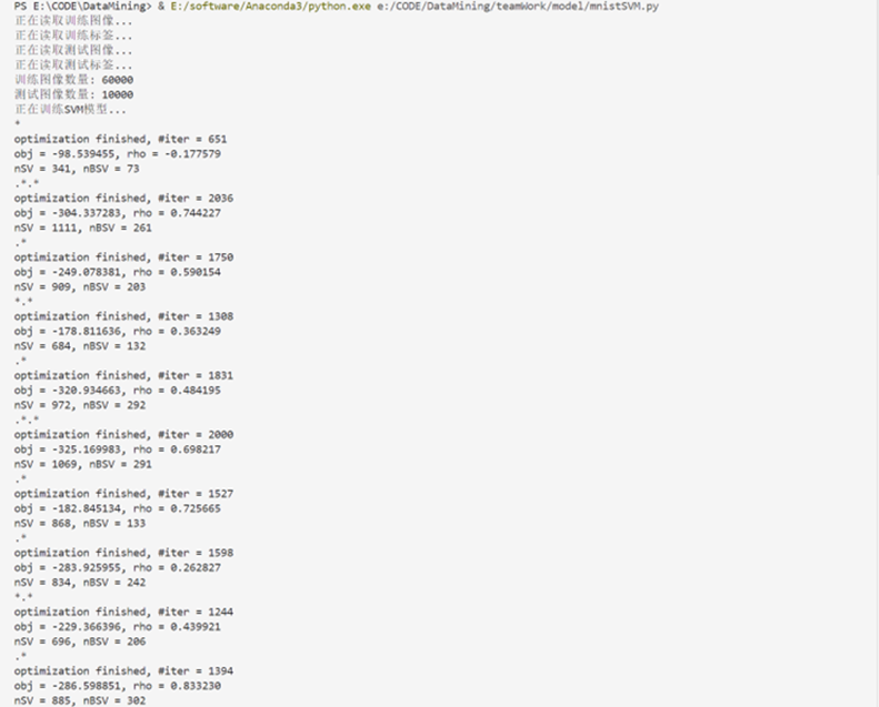
print(“正在训练SVM模型…”)
svm.fit(train_images_flat, train_labels)
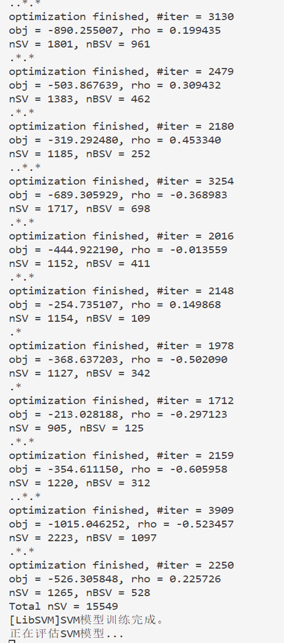
print(“SVM模型训练完成。”)
# 评估模型
print(“正在评估SVM模型…”)
test_predictions = svm.predict(test_images_flat)
test_accuracy = accuracy_score(test_labels, test_predictions)
print(f”\n测试准确率: {test_accuracy}”)
# 打印分类报告
print(“\n分类报告:”)
print(classification_report(test_labels, test_predictions, target_names=[str(i) for i in range(10)]))
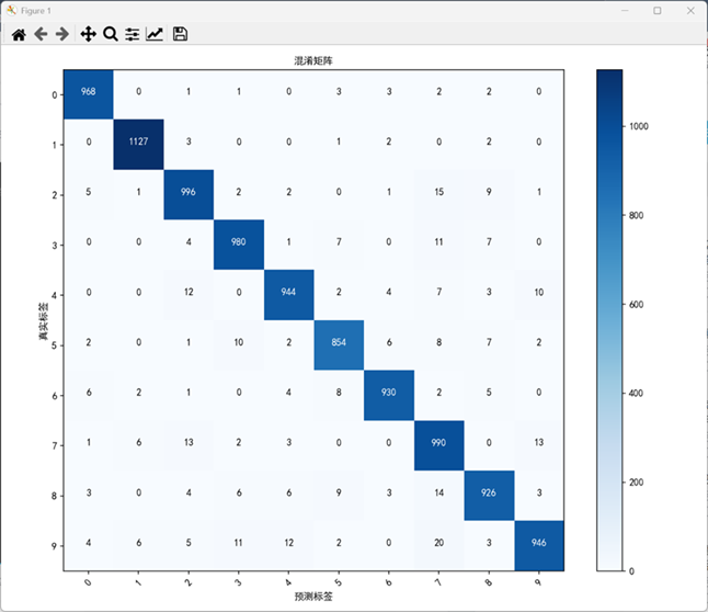
# 混淆矩阵
cm = confusion_matrix(test_labels, test_predictions)
plt.figure(figsize=(10, 8))
plt.imshow(cm, interpolation=’nearest’, cmap=plt.cm.Blues)
plt.title(‘混淆矩阵’, fontproperties=’SimHei’)
plt.colorbar()
tick_marks = np.arange(10)
plt.xticks(tick_marks, [str(i) for i in range(10)], rotation=45, fontproperties=’SimHei’)
plt.yticks(tick_marks, [str(i) for i in range(10)], fontproperties=’SimHei’)
# 在每个单元格上显示数字
thresh = cm.max() / 2.
for i in range(cm.shape[0]):
for j in range(cm.shape[1]):
plt.text(j, i, format(cm[i, j], ‘d’),
horizontalalignment=”center”,
color=”white” if cm[i, j] > thresh else “black”,
fontproperties=’SimHei’)
plt.ylabel(‘真实标签’, fontproperties=’SimHei’)
plt.xlabel(‘预测标签’, fontproperties=’SimHei’)
plt.tight_layout()
plt.show()
# 保存SVM模型
model_save_path = ‘mnist_svm_model.joblib’
joblib.dump(svm, model_save_path)
print(f”模型已保存为 {model_save_path}”)
# 加载并使用保存的SVM模型(示例)
# loaded_svm = joblib.load(model_save_path)
# example_image = test_images_flat[0].reshape(1, -1)
# example_prediction = loaded_svm.predict(example_image)
# print(f”加载的模型预测结果: {example_prediction[0]}, 真实标签: {test_labels[0]}”)
~~~
运行结果:
3.2处理手写数字图片数据集
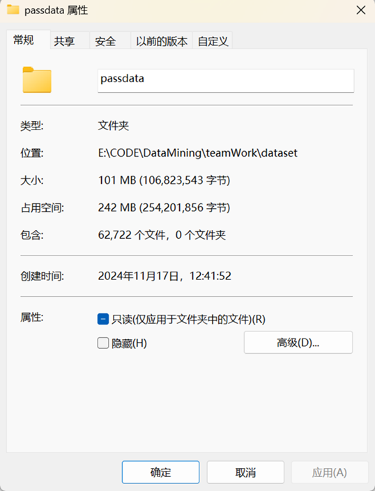
3.2.1 预处理数据集(数据标注)
先将所有图片切片后数据清洗并打标记,剔除不符合规范的图片
3.2.2 KNN(K-近邻算法)
~~~

python代码:

import os

import re

import numpy as np

from sklearn.model_selection import train_test_split

from sklearn.neighbors import KNeighborsClassifier

from sklearn.metrics import accuracy_score

from PIL import Image

# 定义符合要求的文件名模式

pattern = re.compile(r"^\d{8}_\d{2}_\d{3}_[0-9]\.(jpg|png)$")

# 指定要搜索的文件目录

directory = r"E:\CODE\DataMining\teamWork\dataset\passdata"

# 创建数据集列表

images = []

labels = []

# 遍历文件列表

for file in os.listdir(directory):

    if pattern.match(file):

        file_path = os.path.join(directory, file)

        # 读取图像并转换为numpy数组

        image = Image.open(file_path).convert("L")  # 转换为灰度图

        image = image.resize((28, 28))  # 调整图像大小

        image = np.array(image).flatten()  # 展平图像

        images.append(image)

        # 提取标签

        label = int(file.split("_")[-1].split(".")[0])

        labels.append(label)

# 转换为numpy数组

images = np.array(images)

labels = np.array(labels)

# 归一化图像数据

images = images / 255.0

# 划分训练集和测试集

X_train, X_test, y_train, y_test = train_test_split(

    images, labels, test_size=0.2, random_state=42

)

# 构建KNN模型

knn = KNeighborsClassifier(n_neighbors=3)

# 训练模型

knn.fit(X_train, y_train)

# 预测测试集

y_pred = knn.predict(X_test)

# 评估模型

accuracy = accuracy_score(y_test, y_pred)

print(f"测试集准确率: {accuracy * 100:.2f}%")

~~~
运行结果:
PS E:\CODE\DataMining\teamWork> & E:/software/Anaconda3/python.exe e:/CODE/DataMining/teamWork/model/datasetKNN.py
测试集准确率: 81.36%
3.2.3 CNN(卷积神经网络)
~~~

python代码:

import os

import re

import shutil

import numpy as np

import tensorflow as tf

from tensorflow.keras.preprocessing.image import ImageDataGenerator

from tensorflow.keras.models import Sequential

from tensorflow.keras.layers import Conv2D, MaxPooling2D, Flatten, Dense

from sklearn.model_selection import train_test_split

from tensorflow.keras.utils import to_categorical

from PIL import Image

# 定义符合要求的文件名模式

pattern = re.compile(r"^\d{8}_\d{2}_\d{3}_[0-9]\.(jpg|png)$")

# 指定要搜索的文件目录

directory = r"E:\CODE\DataMining\teamWork\dataset\passdata"

# 创建数据集列表

images = []

labels = []

# 遍历文件列表

for file in os.listdir(directory):

    if pattern.match(file):

        file_path = os.path.join(directory, file)

        # 读取图像并转换为numpy数组

        image = Image.open(file_path).convert("L")  # 转换为灰度图

        image = image.resize((28, 28))  # 调整图像大小

        image = np.array(image)

        images.append(image)

        # 提取标签

        label = int(file.split("_")[-1].split(".")[0])

        labels.append(label)

# 转换为numpy数组

images = np.array(images)

labels = np.array(labels)

# 归一化图像数据

images = images / 255.0

# 划分训练集和测试集

X_train, X_test, y_train, y_test = train_test_split(

    images, labels, test_size=0.2, random_state=42

)

# 将标签转换为one-hot编码

y_train = to_categorical(y_train, num_classes=10)

y_test = to_categorical(y_test, num_classes=10)

# 构建CNN模型

model = Sequential(

    [

        Conv2D(32, (3, 3), activation="relu", input_shape=(28, 28, 1)),

        MaxPooling2D((2, 2)),

        Conv2D(64, (3, 3), activation="relu"),

        MaxPooling2D((2, 2)),

        Flatten(),

        Dense(128, activation="relu"),

        Dense(10, activation="softmax"),

    ]

)

# 编译模型

model.compile(optimizer="adam", loss="categorical_crossentropy", metrics=["accuracy"])

# 训练模型

model.fit(X_train, y_train, epochs=10, batch_size=32, validation_data=(X_test, y_test))

# 评估模型

loss, accuracy = model.evaluate(X_test, y_test)

print(f"测试集准确率: {accuracy * 100:.2f}%")

~~~
运行结果:
PS E:\CODE\DataMining\teamWork> & E:/software/Anaconda3/python.exe e:/CODE/DataMining/teamWork/model/datasetCNN.py
2024-11-28 17:45:35.358463: I tensorflow/core/util/port.cc:153] oneDNN custom operations are on. You may see slightly different numerical results due to floating-point round-off errors from different computation orders. To turn them off, set the environment variable `TF_ENABLE_ONEDNN_OPTS=0`.
2024-11-28 17:45:37.022833: I tensorflow/core/util/port.cc:153] oneDNN custom operations are on. You may see slightly different numerical results due to floating-point round-off errors from different computation orders. To turn them off, set the environment variable `TF_ENABLE_ONEDNN_OPTS=0`.
C:\Users\yanyifan\AppData\Roaming\Python\Python312\site-packages\keras\src\layers\convolutional\base_conv.py:107: UserWarning: Do not pass an `input_shape`/`input_dim` argument to a layer. When using Sequential models, prefer using an `Input(shape)` object as the first layer in the model instead.
super().__init__(activity_regularizer=activity_regularizer, **kwargs)
2024-11-28 17:46:23.334702: I tensorflow/core/platform/cpu_feature_guard.cc:210] This TensorFlow binary is optimized to use available CPU instructions in performance-critical operations.
To enable the following instructions: AVX2 FMA, in other operations, rebuild TensorFlow with the appropriate compiler flags.
Epoch 1/10
1569/1569 ━━━━━━━━━━━━━━━━━━━━ 9s 5ms/step – accuracy: 0.5946 – loss: 1.2190 – val_accuracy: 0.9090 – val_loss: 0.3386
Epoch 2/10
1569/1569 ━━━━━━━━━━━━━━━━━━━━ 7s 4ms/step – accuracy: 0.9334 – loss: 0.2623 – val_accuracy: 0.9507 – val_loss: 0.2004
Epoch 3/10
1569/1569 ━━━━━━━━━━━━━━━━━━━━ 7s 4ms/step – accuracy: 0.9534 – loss: 0.1836 – val_accuracy: 0.9564 – val_loss: 0.1807
Epoch 4/10
1569/1569 ━━━━━━━━━━━━━━━━━━━━ 7s 4ms/step – accuracy: 0.9638 – loss: 0.1413 – val_accuracy: 0.9597 – val_loss: 0.1630
Epoch 5/10
1569/1569 ━━━━━━━━━━━━━━━━━━━━ 7s 4ms/step – accuracy: 0.9700 – loss: 0.1135 – val_accuracy: 0.9641 – val_loss: 0.1381
Epoch 6/10
1569/1569 ━━━━━━━━━━━━━━━━━━━━ 7s 4ms/step – accuracy: 0.9743 – loss: 0.0976 – val_accuracy: 0.9601 – val_loss: 0.1460
Epoch 7/10
1569/1569 ━━━━━━━━━━━━━━━━━━━━ 7s 4ms/step – accuracy: 0.9783 – loss: 0.0786 – val_accuracy: 0.9640 – val_loss: 0.1399
Epoch 8/10
1569/1569 ━━━━━━━━━━━━━━━━━━━━ 7s 4ms/step – accuracy: 0.9817 – loss: 0.0673 – val_accuracy: 0.9652 – val_loss: 0.1413
Epoch 9/10
1569/1569 ━━━━━━━━━━━━━━━━━━━━ 7s 4ms/step – accuracy: 0.9837 – loss: 0.0531 – val_accuracy: 0.9653 – val_loss: 0.1404
Epoch 10/10
1569/1569 ━━━━━━━━━━━━━━━━━━━━ 6s 4ms/step – accuracy: 0.9850 – loss: 0.0490 – val_accuracy: 0.9650 – val_loss: 0.1370
393/393 ━━━━━━━━━━━━━━━━━━━━ 1s 1ms/step – accuracy: 0.9639 – loss: 0.1392
测试集准确率: 96.50%
3.2.4 SVM(支持向量机)
~~~

python代码:

import os

import re

import numpy as np

from sklearn.model_selection import train_test_split

from sklearn.svm import SVC

from sklearn.metrics import accuracy_score

from PIL import Image

# 定义符合要求的文件名模式

pattern = re.compile(r"^\d{8}_\d{2}_\d{3}_[0-9]\.(jpg|png)$")

# 指定要搜索的文件目录

directory = r"E:\CODE\DataMining\teamWork\dataset\passdata"

# 创建数据集列表

images = []

labels = []

# 遍历文件列表

for file in os.listdir(directory):

    if pattern.match(file):

        file_path = os.path.join(directory, file)

        # 读取图像并转换为numpy数组

        image = Image.open(file_path).convert("L")  # 转换为灰度图

        image = image.resize((28, 28))  # 调整图像大小

        image = np.array(image).flatten()  # 展平图像

        images.append(image)

        # 提取标签

        label = int(file.split("_")[-1].split(".")[0])

        labels.append(label)

# 转换为numpy数组

images = np.array(images)

labels = np.array(labels)

# 归一化图像数据

images = images / 255.0

# 划分训练集和测试集

X_train, X_test, y_train, y_test = train_test_split(

    images, labels, test_size=0.2, random_state=42

)

# 构建SVM模型

svm = SVC(kernel="linear")

# 训练模型

svm.fit(X_train, y_train)

# 预测测试集

y_pred = svm.predict(X_test)

# 评估模型

accuracy = accuracy_score(y_test, y_pred)

print(f"测试集准确率: {accuracy * 100:.2f}%")

~~~
运行结果:
PS E:\CODE\DataMining\teamWork> & E:/software/Anaconda3/python.exe e:/CODE/DataMining/teamWork/model/datasetSVM.py
加载图像: 100%|████████████████████████████████████████████████████████| 62722/62722 [00:40<00:00, 1556.75it/s]
开始训练模型…
模型训练完成 测试集准确率: 61.73%